I’ll show you how to use bootstrapping, a powerful sampling technique which can be used to estimate confidence bounds, p-values and distributions for samples without the need to model (or understand) the underlying distributions.

Who is this post for?

Have you ever needed to:

1. Find confidence bounds for a weird/complex calculation?
2. Find p-values for an A/B test with an unusual distribution or complex metric calculation?
3. Find p-values for an A/B test with simple distributions and been too lazy to check what hypothesis test to use?

If you answered yes to any of the above, then this post is for you!

Intro

In this post, I hope to:

1. Get you wildly excited about the strengths of bootstrapping.
2. Explain some of the use cases for it.
3. Give a clear, intuitive description of what it is and how it works.
4. Give some example code to show how to carry out bootstrapping.
5. Discuss some of the risks and pitfalls.
6. Refer to some good resources where you can learn more.

A quick aside about why I fell in love with bootstrapping

(if you just want get straight to the technical details, feel free to jump ahead)

Some years ago (reasonably early in my career - probably in 2018 or so), when I was working on some kind of forecasting project, where we were attempting to forecast something like sales volumes or stock levels or occupancy levels or the like, we came across an interesting quandary. We had very limited historic training data, and so had relatively little confidence in the forecasts. We used a collection of different predictive models (including, if memory serves, ARIMA-style models, some linear and logistic regression ones, and eventually a NN), and blended the predictions.

The issue was that we needed to explain to our client just how confident we were (or weren’t) in the forecasts.

While each model (or most at least) that we built had the ability to produce confidence bounds, these seemed far too tight, given how much volatility we could see in the historic data.

We¹ hit on a good idea (although one with questionable justification, which I’ll address below). That idea was to train a set of simple neural networks (NNs) on subsets of the data, and then use the distribution of the predictions of these NNs to create some nice shaded regions around the forecasts we were giving. We knew that NNs behaved weirdly in regression settings when extrapolating, and that this was ‘stochastic’ (in this sense just very sensitive to the initial node weights and the training data).

This did exactly what we wanted - we had nice graphs to show the client which gave a visual demonstration of our reasonably low confidence.

However, it was also wrong, for a few reasons:

1. We had no principled way to choose how to subset the data when training the iterations of the NN. We knew that using small subsamples gave wider prediction bounds, but didn’t know what the right size was.
2. While the shaded areas we could put on the plots were useful, they had no objective meaning.
3. (And finally, we were actually trying to show model uncertainty - e.g. we were essentially assuming some kind of data structure when using a linear model, and we didn’t actually have high confidence that this forecasting problem was a linear one. Bootstrapping doesn’t help here directly, but it helped in a hand-wavy way).

And that’s where the story ended, for a few years.

And then, in 2021 or 2022, I came across bootstrapping, and my life changed for good.

What is bootstrapping

We can phrase this in a few ways, at least one of which will make sense to you, depending on your background and experience (hopefully!):

1. Bootstrapping is a non-parametric way to estimate a population measure from a sample.
2. Bootstrapping is an algorithm which gives equally likely outcomes for some sampled outcome, as if you resampled from scratch.

In short, bootstrapping is an approach (or algorithm) for estimating some measure of some population, based solely on the sample we have available.

Some examples where bootstrapping may be helpful

1. You’ve run an A/B test. What range of uplift values might you expect?
   This is another way of saying: “if we ran this experiment over and over again, what range of uplift values would we expect to see?”
2. We fit a model to some data, where the coefficients in the model have some physical interpretation. What range of coefficient values should we expect to see if we retrained the model on new data?
3. We calculate some business metric (e.g. average cost per order) and would like to know how much this might vary for the next month.

Hopefully you can see where this is going. Anytime we calculate a thing based on a sample of data from some population, and we’re interested to know what the distribution of this thing is, then bootstrapping can help.

How would this traditionally be solved?

For each of the examples mentioned above, there are standard, robust approaches to estimating these things without resorting to bootstrapping.

Specifically for the above:

1. We can pick an appropriate hypothesis test, based on what we know about the distribution. This will allow us to calculate a p-value, and some confidence bounds. In some cases, this can be quite challenging (if either it’s a complex distribution, an unknown distribution, or you don’t know lots of stats) - see this post for more details.
2. Depending on the model you’re fitting, it may have a way to calculate confidence bounds on its coefficients directly (e.g. the Python statsmodel linear regression models have a conf_int method, which will directly return confidence bounds. This is based on the Student’s t-distribution²). Sometimes though, there will either be no way to calculate these confidence bounds, or you may not know how to do it, or even implement it.
3. If we know how this measure is distributed, we can estimate this by using some stats directly (but this only works if the distribution is “well behaved”).

So, while there are sometimes approaches to solving these problems using some stats knowledge, sometimes we either can’t, or don’t know enough to know how.

In these cases, bootstrapping to the rescue!

So, what exactly is bootstrapping?

Bootstrapping relies on being able to use the sample you have to generate equally likely samples (hence the term ‘bootstrapping’, as in pulling yourself by your own bootstraps).

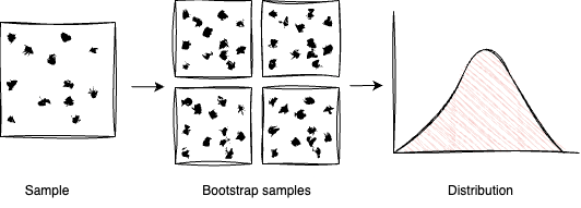
So, we generate lots (usually 1000s) of bootstrap samples from our data. We pretend that each of these is actually a new sample. We calculate the thing on it, and this forms a distribution we can use for whatever we want (getting p-values, confidence bounds, plotting etc).

The magic piece of this is how you generate the bootstrap samples, and this is by sampling with replacement.

So, the process is as follows:

1. Take your sample data, generate $n$ samples with replacement (of the same size of the original data).*
2. For each of these samples, calculate the thing you care about.
3. Use this however you want.

An example in code

Below is some sample code for how to apply the bootstrap process to estimate the distribution and 90% confidence bounds for the mean value of a uniform distribution.

It’s worth noting that the complexity of the run_bootstrap function is seldom more complex than this for most applications (in my experience at least).

import numpy as np
from tqdm import tqdm  # Just to get nice progress meters


# A function which computes a measure (in this case a mean value)
def calculate_measure(data):
    return data.mean()


def run_bootstrap(sample_data, num_iter=1000):
    bootstrap_measures = np.empty(shape=0)
    for _ in tqdm(range(num_iter)):
        bootstrap_sample = np.random.choice(sample_data, size=sample_data.size, replace=True)
        bootstrap_measure = calculate_measure(bootstrap_sample)
        bootstrap_measures = np.append(bootstrap_measures, bootstrap_measure)
    
    return bootstrap_measures


# We have some data that was sampled from somewhere (we'll make some up)
np.random.seed(1)

samples = np.random.random(478)  # We have a set of 478 samples from the population, drawn from the uniform distribution

bootstrap_measures = run_bootstrap(samples)

# We now have a distribution of the sample mean, we can do whatever we want
print(f"Expected value: {bootstrap_measures.mean()}")
print(f"90% confidence bounds: {np.quantile(bootstrap_measures, [0.05, 0.95])}")

When you run this, you’ll get the following:

100%|██████████| 1000/1000 [00:00<00:00, 36131.32it/s]
Expected value: 0.5075680220514992
90% confidence bounds: [0.48611194 0.52922992]

Nothing too surprising here:

1. The expected value of this distribution from the bootstrap estimation is 0.508, where the true value is 0.5 (knowing what we know about the distribution the sample was drawn from).
2. The 90% confidence bounds are wrapped tightly around 0.5. The interpretation for this is: “if we had to draw new samples from the population, and recalculate the mean, 90% of the time these would be between these two values”.

Why does bootstrapping work?

In this section I will give an intuitive explanation of why redrawing samples with replacement works.

One of the best explanations I’ve seen is the answer on this Cross Validated post, which I’ll paraphrase here.

You’d like to ask some question of the population (typically the value of some measure, e.g. what is the average value). You don’t have access to the population, you only have access to the sample. So, instead you ask this same question of the sample. How much confidence should you have that this measure calculated on the sample matches what you would have got if you’d calculated it on the population?

Ideally you’d redraw samples over and over again from the population, and generate a distribution.

But, you don’t have access to the population. Instead, you have two options:

Option 1: Make some assumption about the shape of the population

This is essentially the traditional approach. You make an assumption about the shape of the population (e.g. that it’s normally distributed). You can then draw samples from your parametric normal distribution, and use these to calculate the distribution of measures. If you choose a “convenient” distribution, you may be able to skip the sampling and just calculate the answers directly.

Option 2: Use the sample you already have to learn something about the shape of the population

If you’re unwilling to make assumptions about the population shape, you can then do something else. You can assume that the shape of the population is best represented by the shape of your sample. As conjugateprior says in their answer I linked above:

This is a reasonable thing to do because not only is the sample you have the best, indeed the only information you have about what the population actually looks like, but also because most samples will, if they’re randomly chosen, look quite like the population they came from. Consequently it is likely that yours does too.

Sampling with replacement is really just a shorthand way of doing the following procedure:

1. We want to make our sample a population we can sample from directly.
2. Ideally we’d make a very large (or infinite) number of copies of the data and sample from these.
3. Sampling from the sample with replacement does an equivalent thing.

It’s also worth being clear that we’re not using bootstrapping to estimate something about the population, we’re using it to learn something about the sampling distribution of the population.

Conclusion

I’ve introduced bootstrapping as a tool to generate equally likely samples from an existing sample, and demonstrated how this can be used to estimate the distribution of the mean value of a uniform distribution.

You can use this in a wide range of settings - whenever you don’t have easy access to more samples from the population, and where you’d like some confidence bounds on some parameter, measure or value.

Have a look at my post on using bootstrapping to analyse A/B tests for another use case. I’ll add some more examples in future.

If you have other good resources for introductions to bootstrapping, please let me know in the comments!

Useful links

1. https://statisticsbyjim.com/hypothesis-testing/bootstrapping/
   This describes bootstrapping and confidence bounds in general (it’s a very useful website for stats for practitioners).
2. https://machinelearningmastery.com/a-gentle-introduction-to-the-bootstrap-method/
   Another gentle introduction to bootstrapping.
3. https://erikjanvankesteren.nl/blog/2018-03-01-baron-bootstrap.html
   Yet another gentle introduction³.
4. https://en.wikipedia.org/wiki/Bootstrapping_(statistics)/
   The Wikipedia entry for bootstrapping is quite useful. It also includes some helpful tricks, for example the smoothed bootstrap.
5. https://stats.stackexchange.com/questions/26088/explaining-to-laypeople-why-bootstrapping-works
   This Cross Validated question has some really nice intuitive explanations of why bootstrapping works.
6. https://stats.stackexchange.com/questions/11210/assumptions-regarding-bootstrap-estimates-of-uncertainty
   This Cross Validated question gives a more thorough treatment of the same question as above (although admittedly most of it went over my head).

Footnotes