In this post I’ll give a hands-on walkthrough showing you how to analyse the impact of an A/B test using bootstrap sampling. I’ll also compare this to the traditional approach, to give you confidence that bootstrapping is working the way we expect.

Intro

For a full introduction to bootstrapping, have a look at my post here.

In this post I will:

1. Give a generic A/B test problem statement.
2. Give a concrete example of this, with some data.
3. Explain what kind of answer we’re looking for.
4. Give the traditional solution to the problem.
5. Do it the bootstrapping way.
6. Compare the two approaches.

A/B tests generic problem statement

The generic problem statement for an A/B test analysis is something like this:

• We’ve run an A/B test, exposing some people to variant A, and some to variant B (also called the control and treatment groups).
• Some of these users went on to do something (the conversion goal).
• We’d like to know whether the intervention (the difference between the control and treatment) caused an increase in this goal (and perhaps we’d also like to know how big an increase it caused).

A concrete A/B testing problem statement

Let’s create a simple scenario here to use as a practical example for the rest of the post.

In our sushi delivery app (Fishful Thinking), we offer users a discount code if they sign up for our newsletter. We currently show them a message with the text “Sign up to our newsletter for 5% off your next order”.

Our marketing team has decided to try optimise this copy, to increase the number of people who sign up for the newsletter. They propose “Dive into exclusive deals by subscribing to our newsletter – our fin-tastic discount code will swim straight into your inbox, creating a wave of savings!” [Thanks ChatGPT].

So, here are the important parts:

1. The control group will get the original copy (“Sign up…”).
2. The treatment group will get the proposed copy (“Dive into…”).
3. Our conversion goal is the rate at which users sign-up for the newsletter.

Right, let’s create some synthetic data for this:

import numpy as np
from numpy.random import random
from tqdm import tqdm

np.random.seed(2024)  # Set the seed for reproducibility

# Specify the metadata of the actual distribution 
# (we wouldn't know this in real life)
n_group = 1000

conversion_control = 0.1
conversion_treatment = 0.1 * 1.1  # There is a 10% uplift

# Create the synthetic sample data (this is what we'd get from
# running the experiment)
# Each of these is a binary outcome: did this user sign up
# when shown the message?
samples_control = random(n_group) <= conversion_control
samples_treatment = random(n_group) <= conversion_treatment

Okay, so we have some (synthetic) data. What kind of answer do we want from it?

Basically, we want to know whether the percentage of people in the treatment group who signed up is greater than the percentage of people in the control group who did so, and if so, is this robust (i.e. would we expect this to hold if we roll it out to all users?). The way we test this is by estimating the probability that this increase occurred by chance (the p-value).

The first part of this is easy, we just calculate the uplift directly:

print(f"Control group conversion rate: {samples_control.mean():.1%}")
print(f"Treatment group conversion rate: {samples_treatment.mean():.1%}")
print(f"Uplift: {samples_treatment.mean()/samples_control.mean()-1:.2%}")

Control group conversion rate: 7.0%
Treatment group conversion rate: 10.8%
Uplift: 54.29%

Good. So there appears to be an uplift (and a big one!). From the experiment, we’ve seen that 7% of our users in the control group sign up, but when we show them the new copy, 10.8% sign up, a 54% increase.

Now, this is a fairly small sample - how likely were we to see this uplift if it were caused by chance (i.e. both variants have the same likelihood of conversion, but more users in the treatment just happened to convert?)

The traditional approach

Okay, so if we didn’t have bootstrapping as a tool, how would we go about solving this the traditional way? For A/B tests, we always use some kind of hypothesis test.

The statistical reasoning we follow is this:

• We propose a null hypothesis (that the difference between the performance of the two variants is due to chance - i.e. our hypothesis is that there is no cause, hence null). This is equivalent to the hypothesis that the results are drawn from the same distribution.
• We test how likely this null hypothesis is (this is the p-value). If it’s sufficiently low, then we can reject this null hypothesis.
• Having rejected the null hypothesis, we assert that our hypothesis is true (that the difference in performance between the variants is due to the intervention).

So, we need a traditional approach to finding the probability of the data given the null hypothesis.

We reach into our toolbox of statistical tests for an appropriate test (or we reach for Google or ChatGPT).

In this case a 1-tailed t-test.

I usually check (or just do) this on a website like AB Testguide (most platforms which offer any kind of A/B testing also give some calculators), since it’s usually quicker than finding the right code to use. So, if this is the standard A/B test where the conversion is a proportion, you can just use one of these online calculators.

If we insist on writing our own code (or have to, for more complex problems):

from scipy.stats import ttest_ind

_, p_val_ttest = ttest_ind(samples_control, samples_treatment, alternative="less")
print(f"The ttest p_val: {p_val_ttest:.2}")

The ttest p_val: 0.0014

So, that was reasonably easy (as long as we knew what test to use). In my case I compared the value against an online calculator to be sure I got the maths right.

The bootstrapping approach

Another approach is to use bootstrapping to estimate this directly.

To give some more intuition for what this is doing (you can also check out my full post here for details on the bootstrapping part of this):

• The p-value is the likelihood that we’d observe an effect size of this magnitude or larger, if these samples are drawn from the same distribution (i.e. that there is no effect).
• The p-value is $Pr(d|H_0)$, the probability of the data sample, given the null hypothesis.
• In practice, when we reject the null hypothesis, we assert our alternate hypothesis. Roughly (i.e. in practice), we’re saying that $p_0 = 1-p_{alt}$ (i.e. as the null hypothesis becomes more likely, our alternative hypothesis becomes less likely).
• With bootstrapping, we can answer something slightly different (but equivalent). We can answer how likely it is that we would see a positive effect size if we repeated this experiment over and over again.
  • So, instead of calculating the p-value, we calculate the confidence interval, $\alpha$.
  • We can then convert this to the p-value using $p=1-\alpha$ (see this post by Jim Frost - these are not the same thing, but they always agree - we’ll see an example of this below)¹.
• So, we generate bootstrap samples to simulate repeating the experiment:
  • Each bootstrap sample is our best guess of what running the experiment again would yield.
  • This distribution over possible outcomes gives our best guess for the range of uplift values we’d expect to see in the wild.
  • We can then draw confidence bounds from this distribution, and then extract the p-value from these.

Let’s look at some code for how this works.

num_iter = 10000
res = []
bootstrap_mean_control = []
bootstrap_mean_treatment = []
for _ in tqdm(range(num_iter)):
   bootstrap_sample_control = np.random.choice(samples_control, size=samples_control.size, replace=True)
   bootstrap_sample_treatment = np.random.choice(samples_treatment, size=samples_treatment.size, replace=True)
   bootstrap_mean_control.append(bootstrap_sample_control.mean())
   bootstrap_mean_treatment.append(bootstrap_sample_treatment.mean())

# Calculate p-value for treatment > control
p_val_bootstrap = np.less_equal(bootstrap_mean_treatment, bootstrap_mean_control).mean()

print(f"bootstrap p_val (with {num_iter} iterations): {p_val_bootstrap}")

fig = go.Figure()
fig.add_trace(go.Histogram(x=bootstrap_mean_control, name="control"))
fig.add_trace(go.Histogram(x=bootstrap_mean_treatment, name="treatment"))
fig.update_layout(barmode='overlay')
fig.update_traces(opacity=0.75)
fig.show()

100%|██████████| 10000/10000 [00:00<00:00, 16228.66it/s]
bootstrap p_val (with 10000 iterations): 0.0017

So, we get a p-value of 0.0017, reasonably close to the p-value calculated from the traditional approach (0.0014).

The key observation here is that we look at what percentage of the bootstrap samples led us to seeing the control beating (or at least tieing with) the variant. This is equivalent to the p-value. We can also plot this, which gives us (in my opinion) far more useful information about the performance of the A/B test.

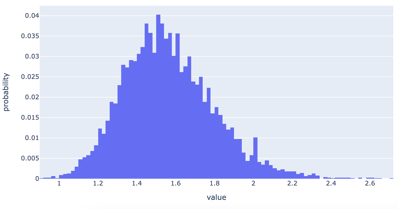
What this shows is our confidence about the possible values of the true uplift. We can see it’s centered around 1.5. But, it also shows how likely it is to be nearer to 1, or 2, or 2.5.

The reason I think this is more useful than a p-value is that instead of just saying whether a positive uplift is likely due to the intervention, it also shows us the magnitude of the probable uplift.

We can go a step further (and should!) to extract from this distribution the confidence intervals. These will be interpreted as the likely range of true uplift values.

## Get some confidence bounds
conf_bounds = np.quantile(np.divide(bootstrap_mean_treatment, bootstrap_mean_control), [0.05, 0.95])
print(f"90% confidence bounds: {conf_bounds}")

90% confidence bounds: [1.21428571 1.98275862]

So, we’re 90% confident that the true uplift value lies between 21% and 98%.

Interestingly, the true value of the uplift (10%) is outside of the 90% confidence bounds. This is because:

1. The sample size (1000) is reasonably small.
2. We were “unlucky” with the specific samples we generated.

You can try changing the seed or increasing the sample size to see what effect this has on the conclusions.

That the true value is outside our confidence bounds should instil a whole lot of caution in how we approach these tests (and stats in general) - we’re just trying to do the best we can, without knowing the truth of the situation. It’s worth adding that the traditional approach has led us to the same conclusions - it’s just the case that we’ve been unlucky with the sample that was drawn. You can look into statistical power, if you’re interested in understanding how to design A/B tests to maximally avoid these kinds of situations.

I’d usually plot these confidence bounds visually, as a really helpful plot to show to stakeholders, because we can use it to reason about the likely impact of rolling out this A/B test.

The useful info this contains:

• We’re 90% confident that the uplift is positive (the entire bar is green).
• We get a sense of the size of the uplift (quite big).

Out of interest, here’s how we’d plot it if the 90% CI includes 0% (which would indicate that the p-value > 0.05).

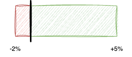
The relative sizes of the red and green bars can be used to make an educated call on whether to roll out the variant or not (going beyond p-values and relying entirely on confidence intervals is beyond the scope of this post, but I may cover it in future).

Conclusion

So, we managed to (closely) replicate the p-value we got from the traditional approach using bootstrapping. Let’s compare:

• Both approaches gave us similar test results - we feel confident rolling out the variant.
• For the traditional approach, we needed to understand the nature of the measure and distributions before knowing which hypothesis test to apply.
• For bootstrapping, it doesn’t matter, we just run the procedure.
• For bootstrapping, we also get confidence intervals and a distribution of the likely uplift values to interpret.

Some interesting things to note about bootstrapping for confidence bounds and p-values

1. The p-value you generate will only have a precision of roughly the inverse of the number of bootstrapping iterations you use. So, if you’d like to evaluate the significance at a level of 0.05, you’ll need at least 20 simulations (and you should always aim for far, far more, given the randomness aspect that affects this).
2. Confidence intervals are similarly affected, since they’re just the quantiles of the bootstrapped measures, so having more bootstrap iterations will make these a little smoother (especially if you want more granular confidence bounds or distributions of the measure).

Useful links:

1. https://statisticsbyjim.com/hypothesis-testing/hypothesis-tests-confidence-intervals-levels/
   Explains that the p-value and confidence intervals always agree.
2. https://statisticsbyjim.com/hypothesis-testing/bootstrapping/
   Describes bootstrapping and confidence bounds.

Footnotes